Deep dive into the whole required stastistics , that would be a required to learn stable diffusion from the very scratch

Probability and Distributions

Probability : It tells the chances of an event to happen. And is calculated as the ratio of no. of outcomes of a particular event to the total no. of outcomes.

Likelihood : It measures how well a statistical model fits the observed data.

Q) What is a statistical model and observed data ?

A) Asssume by tossing a coin 100 times we got 90 heads and 10 tails.

In the coin toss, the statistical model are fair-coin, slightly biased coin, heavily biased coin.

For each model we calculate the likelihood, how probable the observed data (coin toss results) is, and select the one with the highest likelihood.

Take it like this : we flipped a fair coin 100 times and it gives heads 90 times and tails 10 times so the likelihood the coin is fair is quite low

When we say maximise the likelihood … we mean to say, we want the best parameters that are accurately predicting the data

Probability goes from model to data (What data do we expect given this model?) Likelihood goes from data to model (What model best explains this data?)

In genAI: The model whose params are most likely to produce the observed data is selected. Means the one with maximum likelihood is selected. The architecture that work on this principle is called Likelihood based Models

Maximum Likelihood Estimation : We have the intialised parameters of the model and we try to maximise the likelihood by updating the parameters. so our cost function looks like : Theta = argmax(P(X|Theta)) , thetas are the parameters of the model

Normal / gaussian Distribution: The bell shaped curve, having mean-mu and the variance-sigma^2 as parameters.

Joint Distributions: The joint distribution of two random variables X and Y is the probability distribution of the pair (X, Y). It describes the probability of all possible combinations of X and Y.

X = The person is a smoker Y = The person has a disease

P(x=smoker, y=disease) = 0.05 P(x=smoker, y=no-disease) = 0.01 P(x=non-smoker, y=disease) = 0.03 P(x=non-smoker, y=no-disease) = 0.91

Marginal Distributions link: Given a known joint distribution of two discrete random variables, say, X and Y, the marginal distribution of either variable – X for example – is the probability distribution of X when the values of Y are not taken into consideration

*P(x=smoker)[Marginal distribution of X] = P(x=smoker, y=disease) + P(x=smoker, y=no-disease) = 0.05 + 0.01 = 0.06

*P(x=non-smoker)[Marginal distribution of X] = P(x=non-smoker, y=disease) + P(x=non-smoker, y=no-disease) = 0.03 + 0.91 = 0.94

*P(y=disease)[Marginal distribution of Y] = P(x=smoker, y=disease) + P(x=non-smoker, y=disease) = 0.05 + 0.03 = 0.08

*P(y=no-disease)[Marginal distribution of Y] = P(x=smoker, y=no-disease) + P(x=non-smoker, y=no- disease) = 0.01 + 0.91 = 0.92

Marginal Likelihood : Called as model evidence is the probability of observing the data under a given model, averaged over all possible parameter values for that model. Marginalizing out all the o ther variables, that means integrating over all the possible values ( all the possible values of the other variables) This is the reason why trying to calculate it, makes the solution intractable

Marginal likelihood is indeed an extension of regular likelihood where we consider a range of possible parameter values rather than just a single set

Its just an extension of the likelihood .. where dont limit ourself to a set of likely distributions rather consider all the possible distributions and average over it

For each possible combination of μ and σ: a) We calculate the likelihood of our data given those specific values. b) We multiply this by the prior probability we assign to those parameter values. We integrate this product over all possible values of μ and σ. The result is a single number representing how well our model explains the data, considering all possible parameter values.

TODO: multiply is used in cross-entropy as well, ( I still don’t know the reason behind it )

Here in generative models we are marginalizing out the latent space, to make the results come out irrespective of the distribution of the latent space …

Stats Example: Instead of just these two models, we’d consider many combinations of means (e.g., 160-180 cm) and standard deviations (e.g., 1-20 cm). We’d calculate the likelihood for each, weight them by their prior probability, and sum all of these up.

Q) What does Marginal means ? A) Marginalizing out means integrate over that variables value … Not taking consideration of that variable … Less variables to consider … The name marginal comes from the fact that the values are written at the margins of the table

Q) How to choose what to marginalize out ? A) Latent variables represent unobserved factors that influence our data. We’re uncertain about their exact values, but we know they exist within a range. Marginalizing allows us to account for all possible values these factors could take.

In statistics, when we’re unsure about a parameter, we often “integrate it out” to remove that uncertainty from our final result. In deep learning, we’re doing the same with the latent space – integrating out our uncertainty about the exact latent representations.

BUT YOU WILL NEVER FIND THIS IN CODE ? WHY ?

The reason is this is theoretical calculations and doing these on hand leads to a final loss function, that the researchers lead .. (finding out a loss function is not that simple ) The loss function (ELBO) encourages the model to learn a good latent space that, when marginalized over, explains the data well. We start with this crazy maths and end at the loss function, so our model can learn what we want it to learn.

Entropy Link

This is best understood using examples Assume 2 machines A and B , that produces coins ( A,B,C,D ) with some probability distribution.

The probability distribution of the coins produced by machine A is given by P(A), P(B), P(C), P(D) The probability distribution of the coins produced by machine B is given by Q(A), Q(B), Q(C), Q(D)

P(A) = 0.25 P(B) = 0.25 P(C) = 0.25 P(D) = 0.25

Q(A) = 0.125 Q(B) = 0.125 Q(C) = 0.250 Q(D) = 0.500

And we are now playing with this machines A and B, we will push a button and machine will produce a coin and we have to guess that by asking minimum no of yes / no questions to the machine.

Lets play with Machine A

Machine A : shrrr ( coin produced is A )

The most efficient way to guess the coin produced is to ask questions based on the probability distribution of the machine A, ask questiosn whihc divide the probability distribution into two equal parts. Q1) Is the coin produced is CD ? No

Q2) Is the coin produced is B ? No

Means the coin produced is A At min. we asked 2 questions to the machine A to guess the coin produced. On average we asked 2 questions to the machine A to guess the coin produced.

Lets play with Machine B

Machine B : shrrr ( coin produced is A )

** Why are we not asking questions in pairs here? We could have asked questions like Is the coin produced is AB ? or Is the coin produced is CD ? **
This is asking question like is the coin produced CD will increase the no. of questions by more … as we know half of the time the coin produced is D … ( This is the only efficient way to ask questions )

Q1) Is the coin produced is D ? No

Q2) Is the coin produced is C ? No

Q3) Is the coin produced is B ? No

Means the coin produced is A At min. we asked 3 questions to the machine B to guess the coin produced. On average we how many questions we need to ask to machine B ?? This cant be said as the probability distribution of the machine B is not uniform …

To understand this we need to understand this in analogous way, think we want to build Machine A and Machine B.

Machine A is the gold standard, it produces coins with the probability distribution P(A), P(B), P(C), P(D)

Take a peg and bounce disks

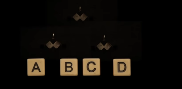
We need to make 2 levels as seen in the above image

For the Machine B :

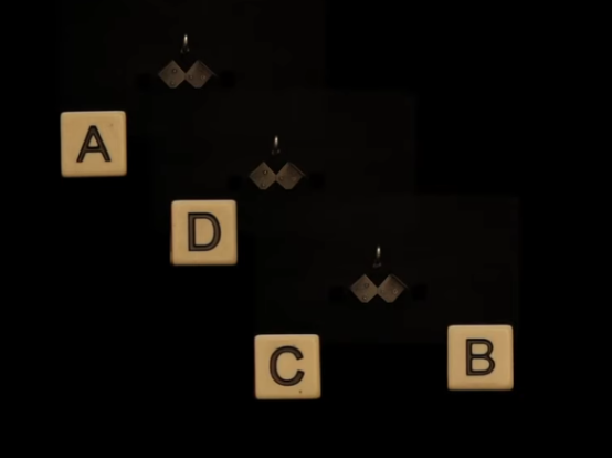
we need to make it to 3 levels

Total no. of bounces can be calculated as weighted probability of the no. of bounces for each level.

Q(A) = 0.125 Q(B) = 0.125 Q(C) = 0.250 Q(D) = 0.500

Total no. of bounces = Q(D) * no_of_levels_down_D_is_present + Q(C) * no_of_levels_down_C_is_present + Q(B) * no_of_levels_down_B_is_present + Q(A) * no_of_levels_down_A_is_present

Total no. of bounces = Q(D) * 1 + Q(C) * 2 + Q(B) * 3 + Q(A) * 3

Total no. of bounces = 0.500 * 1 + 0.250 * 2 + 0.125 * 3 + 0.125 * 3 = 1.75

No. of bounces = No. of questiosn

Machine A requires 2 questions to guess the coin produced Machine B requires 1.75 questions to guess the coin produced

Machine B produces less information hence less uncertainity (if a thing is more certain to happen we automatically have ask less information to confirm it irl )

this measure of Certainity is the called the entropy of the probability distribution

Entropy = - sum ( P(x) * No. of bounces ) [same as above formula]

more specifically no. of bounces are inversely proportional to the probability of that event occuring and that is = log(outcomes at that level)

= log(1/P(x))

which makes entropy = sum ( P(x) * log(1/P(x)) ) or = - sum ( P(x) * log(P(x)) )

Entropy is the amount of information needed to describe the outcome of a random variable / remove the uncertainty of a random variable

In short, whenever the outcomes are equally probable entropy is high and if the outcomes are not equally probable entropy becomes low .. ( not that much intuitive but just the math works !)

Cross-Entropy ( not yet intutive , need to research more on it )

Imagine we’re trying to predict the weather for the next day in a certain city. For simplicity, let’s say there are only three possible weather conditions: Sunny, Rainy, or Cloudy.

True Distribution (P): Let’s say based on historical data, the actual probabilities of these weather conditions are:

Sunny: 50% (0.5) Rainy: 30% (0.3) Cloudy: 20% (0.2)

This is our “true” distribution P.

Predicted Distribution (Q): Now, suppose a meteorologist makes a prediction for tomorrow’s weather:

Sunny: 40% (0.4) Rainy: 35% (0.35) Cloudy: 25% (0.25)

This is our predicted distribution Q.

Now, cross entropy tells us, If we use meterologist guesses to make predictions, how surprised will we be on average when we see the actual weather?

If the meterologist guesses are close to the actual distribution, cross entropy will be low because we’ll be surprised less when we see the actual weather. If the meterologist guesses are far from the actual distribution, cross entropy will be high because we’ll be surprised more when we see the actual weather.

High suprise means more entropy and more no. of bits As the units of suprise / entropy is bits

If the event is more probable, then we require less information about it and vice versa
so information of event = -log(px)

Assume a case like this

Q_ The true prob for a event x = 0.125 , the q(x) = 0.125 then px * logqx = 0.125 ** 3 = 0.375

whereas px = 0.125 and qx = 0.500 then px * logqx = 0.125 * *1 = > 0.125

which means I am getting more surprised when the actual and predicted distribution are same compared to actaul and predicted are different ?

A_ When the event with such low probability actually occurs, it gives more surprise and more no. of bits. When a more probable event occurs it gives less surprise hence less no. of bits.. but in the summation makes things even and the different prob. distributions gives more suprise

Case 1: P matches Q
P(x) = Q(x) = 0.125, P(not-x) = Q(not-x) = 0.875 Cross-entropy = -[0.125 * log₂(0.125) + 0.875 * log₂(0.875)] ≈ 0.544

Case 2: P differs from Q
P(x) = 0.125, Q(x) = 0.500, P(not-x) = 0.875, Q(not-x) = 0.500 Cross-entropy = -[0.125 * log₂(0.500) + 0.875 * log₂(0.500)] = 1.000

KL-Divergence ( once you understand the above two concepts , this is very easy )

KL-Divergence = Cross entropy - Entropy

Entropy: The inherent unpredictability of the weather in your area. Some places have more variable weather (high entropy) than others.

Cross-entropy: How surprised you are by the actual weather, based on your predictions. If your predictions are way off, you’ll be very surprised (high cross-entropy).

KL Divergence: The extra surprise you experience because your predictions aren’t perfect. It’s how much more often you’re caught without an umbrella (or with an unnecessary umbrella) compared to if you had perfect knowledge of the weather patterns.

Closed form solution for KLD LINK

True : data-distribution ( unknown aka multi-variate gaussian distribution i.e. assumption so that we can use closed form solution) Trying to make it : Normal distribution / gaussian distribution